Research - (2023) Volume 12, Issue 5
Bayesian analysis of mammalian animals
Mehari Gebre Teklezgi*,
Abebech Abera Asres,
Gutu Adugna Dabale,
Agnes Matope and
Midaso Bona Wako
Department of Statistics, Adigrat University, Ethiopia
*Correspondence:
Mehari Gebre Teklezgi, Department of Statistics, Adigrat University,
Ethiopia,
Tel: 251947476259,
Email:
Received: 08-Sep-2023, Manuscript No. IPJBS-23-14081;
Editor assigned: 11-Sep-2023, Pre QC No. P-14081;
Reviewed: 27-Sep-2023, QC No. Q-14081;
Revised: 06-Oct-2023, Manuscript No. R-14081;
Published:
16-Oct-2023
Abstract
Growth curve modelling which is a polular methodological tool due to its flexibility. The presence of many wild rabbits, the Oryctolagus cuniculus, in Australia are of major concern. Researchers were interested to investigate the age of the rabbits. Different types of models, including non-linear models were used. Besides, different types of plots and diagrams for the measures of efficiency were used. Results revealed that dry weight of eye lens of the rabbit has nonlinear relationship with the age of the rabbit. The different posterior summary measures shown that differences between the estimates of the models were shown.
Keywords
Bayesian analysis, Rabbit, Growth curve
Introduction
This study is about a Bayesian growth curve model for
rabbit animal. Growth curve modeling, which is a popular
methodological tool due to its flexibility in simultaneously
analyzing both within-animal effects (e.g., assessing change
over time for one animal) and between-animal effects (e.g.,
comparing differences in the change trajectories across
animals).
The presence of many wild rabbits, i.e. the Oryctolagus
cuniculus, in Australia are of major concern. To have more
knowledge on this plague, researchers are interested to
determine the age of the rabbits. While before the weight
of the rabbit was used as a predictor of the age, the dry
weight of the eye lens of the rabbit was proposed as a
more reliable method of age determination. Therefore, a
study was set up, where they measured the dry weight of
the eye lens for free-living wild rabbits of known age [1].
Materials and Methods
Data description: 72 observations from the slightly modified dataset of rabbit with two variables were given.
Age: Age of rabbit in days a covariate.
Lens: Dry weight of eye lens in milligrams as a response.
Exploratory data analysis: As depicted in Tab.1, the age in days has a mean of 240 and standard deviation of 212.7826 with a minimum and maximum days 2,860 respectively. Whereas that of dry weight of the lens has a mean of 143.37 and standard deviation of 67.16638 in milligrams with minimum and maximum of -2.88, 246.70 respectively [2].
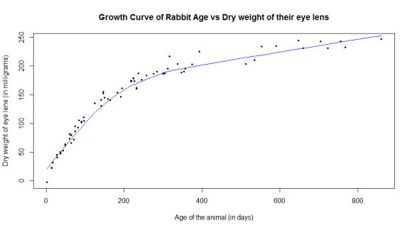
Fig. 1 shows that the growth of dry weight of the eye lens by age (days) are not adequately characterized by a straight line-that is the growth of the rabbit is not linear. Instead, the growth proceed through a number of phases. In the first phase the growth of the animal highly increased, and then after the growth becomes stable, and stable towards a final asymptote. To model growth of the rabbit dry weight in eye lens by age properly, a statistical model must accommodate the nonlinear growth pattern [3].
| Variable |
Minimum |
Median |
Mean |
SD |
Maximum |
| Age |
2.00 |
193.5 |
240.00 |
212.7826 |
860.00 |
| Lens |
-2.88 |
177.64 |
143.37 |
67.16638 |
246.70 |
Tab.1: Descriptive statistics for rabbit data.

Figure 1: Dry weight of eye lens versus age.
Results and Discussion
Model fitting 1: Th first nonlinear model Suggested
for rabbit dataset is given as below.

Where, α, β and γ unknown parameters and £ a normally
distributed error term with constant variance (σ²). In this
model, LENSi is the response measured for the rabbit
i=1, ...71 and Agei the age (days) in which dry weight of
eye lens were measured i=1, ...71 observation. Before the
model was fitted for the final analysis, data was cleaned by
removing one observation that have negative value since
the dry weight of eye lens could not be negative. Before
we remove it, we did the analysis with and without that
observation, and we obtained that the estimates have no difference at all. Then the final analysis was done with 71
observations [4].
This model was fitted using vague priors for all model
parameters and by taking three chains for each parameter.
The convergence of the model was then assessed as
presented by history plots after 50000 itp erations with
burn in period of 20000 and Brooks-Gelman-Rubin
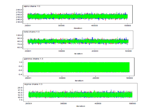
(BGR) Diagnostic as shown in Fig. 2 and 3. The history
plots in Fig. 2 show quite a different sampling behavior for
the regression parameter than γ parameter. The plots for
the regression parameters exhibit slow mixing, but there is
rapid mixing for the γ parameter. The posterior distribution
is therefore rapidly explored in the direction of γ but slowly
explored in the α; β; σ-subspace relatively. However, after
forgetting their starting values, the parameters evolves to a
relatively stable pattern [5].

Figure 2: History plot.

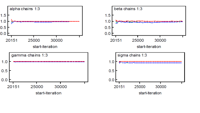
Figure 3: Brooks-Gelman-Rubin
diagnostic.
The Gelman-Rubin convergence diagnostic test also shows
that the chain converged for all regression parameters as
shown in Fig. 3 for all parameters the estimated Potential
Scale Reduction Factor (PSRF) are less than 1.1 or 1.2
which implies the chains are mixing well and the posterior
distribution were converged.
The efficiency of MCMC method can be measured by
the ratio of MC Standard Error (MCSE) to the Standard
Deviation (MCSE/SD). MCSE/SD gives the posterior
variability due to MCMC simulation (Tab. 2).
| |
SD |
MCSE |
MCSE/SD |
Effect sample size |
| Parameters |
3.965 |
0.04365 |
0.0110 |
22000 |
| α |
3.157 |
0.03996 |
0.0126 |
14000 |
| β |
0.1429 |
5.798E-04 |
0.0042 |
20000 |
| ϒ |
1.078 |
0.003781 |
0.0035 |
90000 |
Tab. 2: Measures of efficiency.
Therefore, it is observed from Tab. 2 that the MCSE=SD
for parameters alpha and beta are about 1%, and for
gamma and sigma are about 0.4% and 0.3% respectively.
The result for the parameters alpha and beta implies
that the posterior variability due to MCMC simulation
in alpha as well as in beta is only 1%, this is suggesting
that the MCMC method is efficient. The same is true for
the parameters gamma and sigma with 0.4% and 0.3%
implying that only 0.4% in gamma and 0.3% in sigma
the posterior variability occurred due to MCMC method,
which is very small variability and is indicating that the
MCMC simulation method is efficient [6].
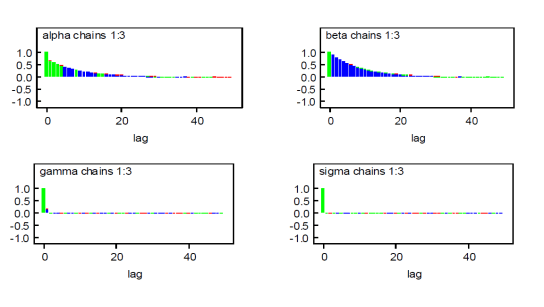
In addition to that it can also be measured by Effective
Sample Size (ESS) and Autocorrelation Function (ACF)
as presented. A high value of the ESS in Tab. 2 implies
that how the MCMC method was efficient, and also the
low autocorrelation presented in Fig. 4 depicted how
the MCMC method was efficient as we can see from the
plot ACF for all parameters is about zero after lag-50. In
conclusion the high ESS and the small ACF implies that
MCMC method was efficient.

Figure 4: Autocorrelation function.
Assumptions of error terms: The residual plot in Fig.
5(a) seems to indicate that the residuals and the fitted
values are in a hoT moscedastic variation with normally
distributed errors. A Q-Q plot in Fig. 5(b) that plotted for
two sets of quantiles against one another shows that the
quantiles came from the same normal distributions [7].

Figure 5: Assumption for error
term.
Moreover, Posterior Predictive Checks (PPC) are used only
as measures of discrepancy between the model and the data
in order to identify poorly fitted models (model adequacy)
and not for model comparison and inference. As the aim
of PPC is to assess the systematic discrepancies between the
observed data and (hypothetical) replicated data generated
from the fitted model, P-values for Skewness and kurtosis
of test statistic and discrepancy measures were given here.
As it was observed from the Tab. 3, the p-values are higher
than 5% significance level except for the Skewness test.
Although Skewness test indicates that there is no goodness
of fit, this was not confirmed by the kurtosis measure of
discrepancy. Therefore, the model fits the data well [8].
| Test |
PTskew |
PDskew |
PTkurt |
PDkurt |
| Estimate |
0.00012 |
0.07850 |
0.99700 |
0.60000 |
Tab. 3: Posterior Predictive Checks (PPC) for checking model adequacy.
The histogram of the kurtosis in Fig. 6 (a) seems that the
concentration of the observation is too much at the center
we can call it Leptokurtic. But the kurtosis discrepancy
measure in Fig. 6 (b) seems the distribution is symmetric
and normal. But the histogram in Fig. 6 (c) is moderately
skewed left, the left tail is longer and most of the
distribution is at the right. Also the measure of Skewness
discrepancy measure seems the distribution of the data is to
one direction as we can see from the Fig. 6 (d). From this
we can conclude that the distribution of the observation by
measure of kurtosis discrepancy seems normal.

Figure 6: Posterior predictive hecks.
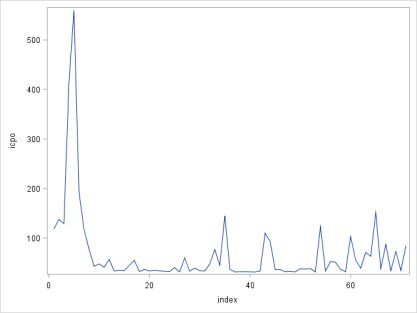
For checking the outlying observations, index plot of icpo
(inverse conditional predictive ordinate) was used (Fig. 7).
Since a small value of iCPO (larger value of CPO) implies
a better fit of the model to a single observation, and large
iCPO valus (low CPO values) suggested that observation
is an outlier and an influential observation. Due to
the face that Inverse-CPO’s (ICPO’s) larger than 40
can be considered as possible outliers, and higher than
70 as extreme values, the index of iCPO pointed that
there seems five possible outlying regions, i.e. regions 6, 36, 44, 55 and 65 might be considered as outlying.
These regions in turn considered of considerable
observations, but possibly region 6 is the extreme region
with about 5 observations [9].

Figure 7: Index plot of iCPO.
Model fitting 2: The second nonlinear model assumed
for the Rabbit data set is given as below.

with α, β and γ unknown parameters and £ a normally distributed error term with constant variance (σ²). In this
model LENS i is the response measured for the rabbit i = 1; :::71 and Age i the age (days) in which dry weight of eye
lens were measured i = 1; :::71 observation.
In order to select the best one from models (1) and,
Deviance Information Criteria (DIC) was used (Tab. 4).
| Model |
DIC |
| Model I |
561.768 |
| Model II |
678.096 |
Tab. 4: The two models and their respective DIC values.
As a very roughly rule of thumb, differences of more than
10 might definitely rule out the model with the higher
DIC. As it is observed in Tab. 4, model 1 is taken as the
best since its DIC value is smaller than that of model 2 and
the difference is clearly visible that is more than 10 (Tab.
5).
| Node |
Mean |
SD |
MC error |
2.50% |
Median |
97.50% |
Start |
Sample |
Model I |
| α |
252.4 |
4.001 |
0.045 |
244.7 |
252.4 |
260.4 |
20001 |
90000 |
| β |
79.69 |
3.189 |
0.042 |
73.58 |
79.63 |
86.14 |
20001 |
90000 |
| ϒ |
0.777 |
0.142 |
5.42E-4 |
0.518 |
0.790 |
0.991 |
20001 |
90000 |
| σ |
12.43 |
1.078 |
0.004 |
10.54 |
12.35 |
14.76 |
20001 |
90000 |
Model II |
| α |
4.507 |
0.039 |
6.80E-4 |
4.43 |
4.507 |
4.586 |
20001 |
90000 |
| β |
115.9 |
15.88 |
0.273 |
87.48 |
114.9 |
150 |
20001 |
90000 |
| ϒ |
0.742 |
0.144 |
5.21E-4 |
0.512 |
0.738 |
0.987 |
20001 |
90000 |
| σ |
28.19 |
2.433 |
0.009 |
23.89 |
28.03 |
33.39 |
20001 |
90000 |
Tab. 5: Posterior summary measures of model 1 and model 2.
It is depicted from Tab. 5 that the estimated values (mean)
and median for α and σ are higher in model I than in model
II, but for β they are higher in model II. The credibility
equal tail interval for respective parameter gives the domain (interval) of the posterior probability of that parameter
estimate. The MC errors are small (smaller than 5% SD) in
all parameters of both models. 20001 and 90000 implies
that 20000 burn-in iterations and 90000 extra iterations
were performed.
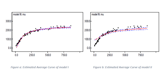
To compare the estimated curves of the two models, Fig. 8 was given below.
Fig. 8 indicated that the fitted average curve for model I
seems to have the better fit as compared to that of model II.

Figure 8: Estimated average
curves of the two models.
Conclusion
In order to have some insight in to the data, descriptive
statistics using tabular and graphical description was
done. From the growth curve it was depicted that the dry
weight of eye lens has a nonlinear relationship with age.
Observing this, two different nonlinear models were fitted
separately using vague priors for all parameters, and taking
three chains their convergence were assessed. Eventually,
as the MC error of each parameter was less than 5% of
its respective standard deviation, well convergence was
observed. Goodness of fit test was done using posterior
predictive checks, and was shown that the model fitted the
data well. Moreover, conditional predictive ordinate was
used to check outlying observations, and some outlying
observations were observed. The two models were compared
using DIC, and model I was chosen as the best model as
it has small DIC. As well, the posterior summary measures
for all the model parameters of models were assessed, and
in some case, differences between the estimates of the two
models were revealed. Choosing model I as the best using
DIC was also confirmed by the estimated average curves.
References
- Lesaffre E, Lawson A. Bayesian Biostatistics. John Wiley and Sons. New York. 2012.
[Google Scholar]
- Duchateau L, Janssen P. The frailty model. Springer Science and Business Media. New York. 2007.
[Google Scholar]
- Ntzoufras I. Bayesian modeling using WinBUGS. John Wiley and Sons. New York. 2009.
[Google Scholar]
- Leache AD, Crews SC, Hickerson MJ. Two waves of diversification in mammals and reptiles of Baja California revealed by hierarchical Bayesian analysis. Biol Lett. 2007;3:646-50.
[Crossref] [Google Scholar] [PubMed]
- Murphy WJ, Eizirik E, O'Brien SJ, et al. Resolution of the early placental mammal radiation using Bayesian phylogenetics. Science. 2001;294:2348-51.
[Crossref] [GoogleScholar] [PubMed]
- Waddell PJ, Kishino H, Ota R. A phylogenetic foundation for comparative mammalian genomics. Genome Inform. 2001;12:141-54.
[Google Scholar] [PubMed]
- Maness HT, Nollens HH, Jensen ED, et al. Phylogenetic analysis of marine mammal herpesviruses. Vet Microbiol. 2011;149:23-9.
[Crossref] [Google Scholar] [PubMed]
- Casellas J, Canas-Alvarez JJ, Gonzalez-Rodriguez A, et al. Bayesian analysis of parent-specific transmission ratio distortion in seven Spanish beef cattle breeds. Anim Genet. 2017;48:93-6.
[Crossref] [Google Scholar] [PubMed]
- Alfellani MA, Taner-Mulla D, Jacob AS, et al. Genetic diversity of Blastocystis in livestock and zoo animals. Protist. 2013;164(4):497-509.
[Crossref] [Google Scholar] [PubMed]


